We return now to the prediction case to take a closer look at the interaction
between bootstrapping, function approximation, and the on-policy distribution.
By bootstrapping we mean the updating of a value estimate on the basis of
other value estimates. TD methods involve bootstrapping, as do DP
methods, whereas Monte Carlo methods do not. TD(![]() ) is a bootstrapping
method for
) is a bootstrapping
method for ![]() , and by convention we consider it not to be a
bootstrapping method for
, and by convention we consider it not to be a
bootstrapping method for ![]() . Although TD(1) involves bootstrapping within an
episode, the net effect over a complete episode is the same as a
nonbootstrapping Monte Carlo update.
. Although TD(1) involves bootstrapping within an
episode, the net effect over a complete episode is the same as a
nonbootstrapping Monte Carlo update.
Bootstrapping methods are more difficult to combine with function approximation than
are nonbootstrapping methods. For example, consider the case of value prediction with
linear, gradient-descent function approximation. In this case, nonbootstrapping
methods find minimal MSE (8.1) solutions for any distribution of training
examples, ![]() , whereas bootstrapping methods find only near-minimal MSE
(8.9) solutions, and only for the on-policy distribution. Moreover, the
quality of the MSE bound for TD(
, whereas bootstrapping methods find only near-minimal MSE
(8.9) solutions, and only for the on-policy distribution. Moreover, the
quality of the MSE bound for TD(![]() ) gets worse the farther
) gets worse the farther ![]() strays from 1, that is,
the farther the method moves from its nonbootstrapping form.
strays from 1, that is,
the farther the method moves from its nonbootstrapping form.
The restriction of the convergence results for bootstrapping methods to the on-policy distribution is of greatest concern. This is not a problem for on-policy methods such as Sarsa and actor-critic methods, but it is for off-policy methods such as Q-learning and DP methods. Off-policy control methods do not backup states (or state-action pairs) with exactly the same distribution with which the states would be encountered following the estimation policy (the policy whose value function they are estimating). Many DP methods, for example, backup all states uniformly. Q-learning may backup states according to an arbitrary distribution, but typically it backs them up according to the distribution generated by interacting with the environment and following a soft policy close to a greedy estimation policy. We use the term off-policy bootstrapping for any kind of bootstrapping using a distribution of backups different from the on-policy distribution. Surprisingly, off-policy bootstrapping combined with function approximation can lead to divergence and infinite MSE.
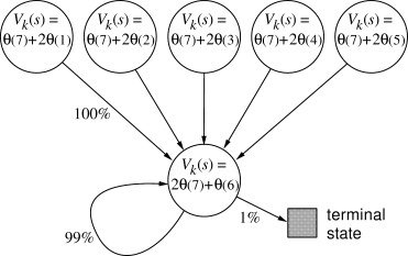
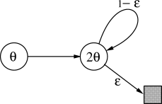
Example 8.3: Baird's Counterexample Consider the six-state, episodic Markov process shown in Figure 8.12. Episodes begin in one of the five upper states, proceed immediately to the lower state, and then cycle there for some number of steps before terminating. The reward is zero on all transitions, so the true value function is
|
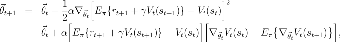
The prediction method we apply to this task is a linear,
gradient-descent form of DP policy evaluation. The parameter vector, ![]() , is
updated in sweeps through the state space, performing a synchronous,
gradient-descent backup at every state,
, is
updated in sweeps through the state space, performing a synchronous,
gradient-descent backup at every state, ![]() , using the DP (full backup) target:
, using the DP (full backup) target:

|
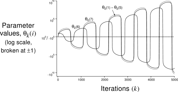
If we alter just the distribution of DP backups in Baird's counterexample, from
the uniform distribution to the on-policy distribution (which generally requires
asynchronous updating), then convergence is guaranteed to a solution with error
bounded by (8.9) for ![]() . This example is striking because the
DP method used is arguably the simplest and best-understood bootstrapping
method, and the linear, gradient-descent method used is arguably the
simplest and best-understood kind of function approximation. The example shows
that even the simplest combination of bootstrapping and function approximation
can be unstable if the backups are not done according to the on-policy
distribution.
. This example is striking because the
DP method used is arguably the simplest and best-understood bootstrapping
method, and the linear, gradient-descent method used is arguably the
simplest and best-understood kind of function approximation. The example shows
that even the simplest combination of bootstrapping and function approximation
can be unstable if the backups are not done according to the on-policy
distribution.
There are also counterexamples similar to Baird's showing divergence for
Q-learning. This is cause for concern because otherwise Q-learning has
the best convergence guarantees of all control methods. Considerable effort has
gone into trying to find a remedy to this problem or to obtain some weaker, but still
workable, guarantee. For example, it may be possible to guarantee convergence of
Q-learning as long as the behavior policy (the policy used to select actions) is
sufficiently close to the estimation policy (the policy used in GPI), for example,
when it is the ![]() -greedy policy. To the best of our knowledge, Q-learning has never
been found to diverge in this case, but there has been no theoretical analysis.
In the rest of this section we present several other ideas that have been
explored.
-greedy policy. To the best of our knowledge, Q-learning has never
been found to diverge in this case, but there has been no theoretical analysis.
In the rest of this section we present several other ideas that have been
explored.
Suppose that instead of taking just a step toward
the expected one-step return on each iteration, as in Baird's
counterexample, we actually change the value function all the way to the best, least-squares
approximation. Would this solve the instability problem? Of course it would
if the feature vectors, ![]() , formed a linearly independent
set, as they do in Baird's counterexample, because then exact approximation is
possible on each iteration and the method reduces to standard tabular DP.
But of course the point here is to consider the case when an exact solution
is not possible. In this case stability is not
guaranteed even when forming the best approximation at each iteration, as shown
by the following example.
, formed a linearly independent
set, as they do in Baird's counterexample, because then exact approximation is
possible on each iteration and the method reduces to standard tabular DP.
But of course the point here is to consider the case when an exact solution
is not possible. In this case stability is not
guaranteed even when forming the best approximation at each iteration, as shown
by the following example.
|
Example 8.4: Tsitsiklis and Van Roy's Counterexample The simplest counterexample to linear least-squares DP is shown in Figure 8.14. There are just two nonterminal states, and the modifiable parameter
One way to try to prevent instability is to use special methods for function approximation. In particular, stability is guaranteed for function approximation methods that do not extrapolate from the observed targets. These methods, called averagers, include nearest neighbor methods and local weighted regression, but not popular methods such as tile coding and backpropagation.
Another approach is to attempt to minimize not the mean-squared error from the
true value function (8.1), but the mean-squared error from the expected
one-step return. It is natural to call this error measure the
mean-squared Bellman error:
|
Exercise 8.9 (programming) Look up the paper by Baird (1995) on the Internet and obtain his counterexample for Q-learning. Implement it and demonstrate the divergence.