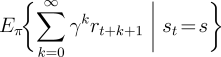
Both TD and Monte Carlo methods use experience to solve the prediction problem.
Given some experience following a policy ![]() , both methods update their estimate
, both methods update their estimate
![]() of
of ![]() . If a nonterminal state
. If a nonterminal state ![]() is visited at time
is visited at time ![]() , then both
methods update their estimate
, then both
methods update their estimate ![]() based on what happens after that visit.
Roughly speaking, Monte Carlo methods wait until the return following the
visit is known, then use that return as a target for
based on what happens after that visit.
Roughly speaking, Monte Carlo methods wait until the return following the
visit is known, then use that return as a target for ![]() . A simple
every-visit Monte Carlo method suitable for nonstationary environments is
. A simple
every-visit Monte Carlo method suitable for nonstationary environments is
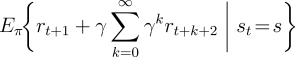
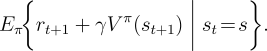
Because the TD method bases its update in part on an existing estimate, we say
that it is a bootstrapping method, like DP. We know from Chapter 3
that
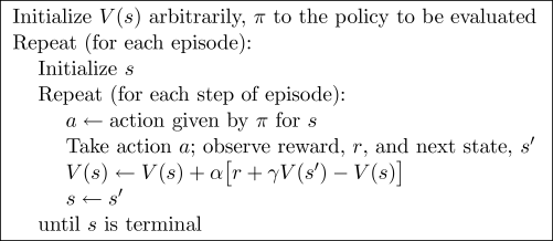
Figure 6.1 specifies TD(0) completely in procedural form, and Figure 6.2 shows its backup diagram. The value estimate for the state node at the top of the backup diagram is updated on the basis of the one sample transition from it to the immediately following state. We refer to TD and Monte Carlo updates as sample backups because they involve looking ahead to a sample successor state (or state-action pair), using the value of the successor and the reward along the way to compute a backed-up value, and then changing the value of the original state (or state-action pair) accordingly. Sample backups differ from the full backups of DP methods in that they are based on a single sample successor rather than on a complete distribution of all possible successors.
Example 6.1: Driving Home Each day as you drive home from work, you try to predict how long it will take to get home. When you leave your office, you note the time, the day of week, and anything else that might be relevant. Say on this Friday you are leaving at exactly 6 o'clock, and you estimate that it will take 30 minutes to get home. As you reach your car it is 6:05, and you notice it is starting to rain. Traffic is often slower in the rain, so you reestimate that it will take 35 minutes from then, or a total of 40 minutes. Fifteen minutes later you have completed the highway portion of your journey in good time. As you exit onto a secondary road you cut your estimate of total travel time to 35 minutes. Unfortunately, at this point you get stuck behind a slow truck, and the road is too narrow to pass. You end up having to follow the truck until you turn onto the side street where you live at 6:40. Three minutes later you are home. The sequence of states, times, and predictions is thus as follows:
| Elapsed Time | Predicted | Predicted | |
| State | (minutes) | Time to Go | Total Time |
| leaving office, friday at 6 | 0 | 30 | 30 |
| reach car, raining | 5 | 35 | 40 |
| exiting highway | 20 | 15 | 35 |
| 2ndary road, behind truck | 30 | 10 | 40 |
| entering home street | 40 | 3 | 43 |
| arrive home | 43 | 0 | 43 |
The rewards in this example are the elapsed times on each leg of the
journey.6.1 We are not
discounting (![]() ), and thus the return for each state is the actual
time to go from that state. The value of each state is the expected
time to go. The second column of numbers gives the current estimated value for each
state encountered.
), and thus the return for each state is the actual
time to go from that state. The value of each state is the expected
time to go. The second column of numbers gives the current estimated value for each
state encountered.
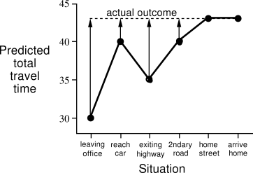
A simple way to view the operation of Monte Carlo methods is to
plot the predicted total time (the last column) over the sequence, as in
Figure
6.3. The arrows show the changes in
predictions recommended by the constant-![]() MC method (6.1), for
MC method (6.1), for
![]() . These are exactly the errors between the estimated value (predicted time
to go) in each state and the actual return (actual time to go). For example,
when you exited the highway you thought it would take only 15 minutes more to get
home, but in fact it took 23 minutes. Equation (6.1) applies at this
point and determines an increment in the estimate of time to go after exiting the
highway. The error,
. These are exactly the errors between the estimated value (predicted time
to go) in each state and the actual return (actual time to go). For example,
when you exited the highway you thought it would take only 15 minutes more to get
home, but in fact it took 23 minutes. Equation (6.1) applies at this
point and determines an increment in the estimate of time to go after exiting the
highway. The error,
![]() , at this time is eight minutes. Suppose the step-size parameter,
, at this time is eight minutes. Suppose the step-size parameter,
![]() , is
, is ![]() . Then the predicted time to go after exiting the highway
would be revised upward by four minutes as a result of this experience. This is
probably too large a change in this case; the truck was probably just an unlucky
break. In any event, the change can only be made off-line, that is, after you
have reached home. Only at this point do you know any of the actual returns.
. Then the predicted time to go after exiting the highway
would be revised upward by four minutes as a result of this experience. This is
probably too large a change in this case; the truck was probably just an unlucky
break. In any event, the change can only be made off-line, that is, after you
have reached home. Only at this point do you know any of the actual returns.
Is it necessary to wait until the final outcome is known before learning can begin? Suppose on another day you again estimate when leaving your office that it will take 30 minutes to drive home, but then you become stuck in a massive traffic jam. Twenty-five minutes after leaving the office you are still bumper-to-bumper on the highway. You now estimate that it will take another 25 minutes to get home, for a total of 50 minutes. As you wait in traffic, you already know that your initial estimate of 30 minutes was too optimistic. Must you wait until you get home before increasing your estimate for the initial state? According to the Monte Carlo approach you must, because you don't yet know the true return.
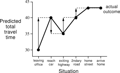
According to a TD approach, on the other hand, you would learn immediately,
shifting your initial estimate from 30 minutes toward 50. In fact, each estimate
would be shifted toward the estimate that immediately follows it. Returning to
our first day of driving, Figure
6.4 shows the same predictions as
Figure
6.3, except with the changes recommended
by the TD rule (6.2) (these are the changes made by the rule if
![]() ). Each error is proportional to the change over time of the prediction,
that is, to the temporal differences in predictions.
). Each error is proportional to the change over time of the prediction,
that is, to the temporal differences in predictions.
Besides giving you something to do while waiting in traffic, there are several computational reasons why it is advantageous to learn based on your current predictions rather than waiting until termination when you know the actual return. We briefly discuss some of these next.