We begin by looking more closely at some simple methods for estimating the
values of actions and for using the estimates to make action selection decisions.
In this chapter, we denote the true (actual) value of action ![]() as
as ![]() ,
and the estimated value at the
,
and the estimated value at the ![]() th play as
th play as ![]() . Recall that the true value
of an action is the mean reward received when that action is selected. One natural
way to estimate this is by averaging the rewards actually received when the
action was selected. In other words, if at the
. Recall that the true value
of an action is the mean reward received when that action is selected. One natural
way to estimate this is by averaging the rewards actually received when the
action was selected. In other words, if at the ![]() th play action
th play action ![]() has been
chosen
has been
chosen ![]() times prior to
times prior to ![]() , yielding rewards
, yielding rewards ![]() , then
its value is estimated to be
, then
its value is estimated to be
The simplest action selection rule is to select the action (or one of the
actions) with highest estimated action value, that is, to select on
play ![]() one of the greedy actions,
one of the greedy actions,
![]() , for which
, for which ![]() . This method
always exploits current knowledge to maximize immediate reward; it spends
no time at all sampling apparently inferior actions to see if they might
really be better. A simple alternative is to behave greedily most of the
time, but every once in a while, say with small probability
. This method
always exploits current knowledge to maximize immediate reward; it spends
no time at all sampling apparently inferior actions to see if they might
really be better. A simple alternative is to behave greedily most of the
time, but every once in a while, say with small probability ![]() , instead
select an action at random, uniformly, independently of the action-value
estimates. We call methods using this near-greedy action selection rule
, instead
select an action at random, uniformly, independently of the action-value
estimates. We call methods using this near-greedy action selection rule
![]() -greedy methods. An advantage of these methods is that, in the limit
as the number of plays increases, every action will be sampled an
infinite number of times, guaranteeing that
-greedy methods. An advantage of these methods is that, in the limit
as the number of plays increases, every action will be sampled an
infinite number of times, guaranteeing that ![]() for all
for all
![]() , and thus ensuring that all the
, and thus ensuring that all the ![]() converge to
converge to ![]() . This of course
implies that the probability of selecting the optimal action converges to
greater than
. This of course
implies that the probability of selecting the optimal action converges to
greater than ![]() , that is, to near certainty. These are just
asymptotic guarantees, however, and say little about the practical effectiveness
of the methods.
, that is, to near certainty. These are just
asymptotic guarantees, however, and say little about the practical effectiveness
of the methods.
To roughly assess the relative effectiveness of the greedy and ![]() -greedy methods, we
compared them numerically on a suite of test problems. This is a set of 2000 randomly
generated
-greedy methods, we
compared them numerically on a suite of test problems. This is a set of 2000 randomly
generated ![]() -armed bandit tasks with
-armed bandit tasks with ![]() . For each action,
. For each action, ![]() , the rewards were
selected from a normal (Gaussian) probability distribution with mean
, the rewards were
selected from a normal (Gaussian) probability distribution with mean ![]() and
variance
and
variance ![]() . The 2000
. The 2000 ![]() -armed bandit tasks were generated by
reselecting the
-armed bandit tasks were generated by
reselecting the ![]() 2000 times, each according to a normal distribution with
mean
2000 times, each according to a normal distribution with
mean
![]() and variance
and variance ![]() . Averaging over tasks, we can plot the performance and
behavior of various methods as they improve with experience over 1000 plays, as in
Figure
2.1. We call this suite of test tasks the 10-armed testbed.
. Averaging over tasks, we can plot the performance and
behavior of various methods as they improve with experience over 1000 plays, as in
Figure
2.1. We call this suite of test tasks the 10-armed testbed.
|
Figure
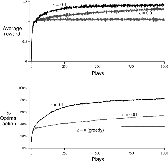
2.1 compares a greedy method with two
![]() -greedy methods (
-greedy methods (![]() and
and ![]() ), as described above, on the 10-armed
testbed. Both methods formed their action-value estimates using the
sample-average technique. The upper graph shows the increase in expected reward
with experience. The greedy method improved slightly faster than the other
methods at the very beginning, but then leveled off at a lower level. It
achieved a reward per step of only about 1, compared with the best possible of
about 1.55 on this testbed. The greedy method performs significantly worse in
the long run because it often gets stuck performing suboptimal actions. The
lower graph shows that the greedy method found the optimal action in only
approximately one-third of the tasks. In the other two-thirds, its initial
samples of the optimal action were disappointing, and it never returned to it.
The
), as described above, on the 10-armed
testbed. Both methods formed their action-value estimates using the
sample-average technique. The upper graph shows the increase in expected reward
with experience. The greedy method improved slightly faster than the other
methods at the very beginning, but then leveled off at a lower level. It
achieved a reward per step of only about 1, compared with the best possible of
about 1.55 on this testbed. The greedy method performs significantly worse in
the long run because it often gets stuck performing suboptimal actions. The
lower graph shows that the greedy method found the optimal action in only
approximately one-third of the tasks. In the other two-thirds, its initial
samples of the optimal action were disappointing, and it never returned to it.
The
![]() -greedy methods eventually perform better because they continue to explore, and
to improve their chances of recognizing the optimal action. The
-greedy methods eventually perform better because they continue to explore, and
to improve their chances of recognizing the optimal action. The
![]() method explores more, and usually finds the optimal action earlier, but never
selects it more than 91% of the time. The
method explores more, and usually finds the optimal action earlier, but never
selects it more than 91% of the time. The ![]() method improves more slowly,
but eventually performs better than the
method improves more slowly,
but eventually performs better than the ![]() method on both performance
measures. It is also possible to reduce
method on both performance
measures. It is also possible to reduce ![]() over time to try to get the best of both
high and low values.
over time to try to get the best of both
high and low values.
The advantage of ![]() -greedy over greedy methods depends on the task. For example,
suppose the reward variance had been larger, say 10 instead of 1. With noisier
rewards it takes more exploration to find the optimal action, and
-greedy over greedy methods depends on the task. For example,
suppose the reward variance had been larger, say 10 instead of 1. With noisier
rewards it takes more exploration to find the optimal action, and ![]() -greedy
methods should fare even better relative to the greedy method.
On the other hand, if the reward variances were zero, then the greedy method would
know the true value of each action after trying it once. In this case the greedy method
might actually perform best because it would soon find the optimal action and then never
explore. But even in the deterministic case, there is a large advantage to exploring if
we weaken some of the other assumptions. For example, suppose the bandit task were
nonstationary, that is, that the true values of the actions changed over time. In this
case exploration is needed even in the deterministic case to make sure one of the
nongreedy actions has not changed to become better than the greedy one. As we
will see in the next few chapters, effective nonstationarity is the case most commonly
encountered in reinforcement learning. Even if the underlying task is stationary
and deterministic, the learner faces a set of banditlike decision tasks each
of which changes over time due to the learning process itself. Reinforcement
learning requires a balance between exploration and exploitation.
-greedy
methods should fare even better relative to the greedy method.
On the other hand, if the reward variances were zero, then the greedy method would
know the true value of each action after trying it once. In this case the greedy method
might actually perform best because it would soon find the optimal action and then never
explore. But even in the deterministic case, there is a large advantage to exploring if
we weaken some of the other assumptions. For example, suppose the bandit task were
nonstationary, that is, that the true values of the actions changed over time. In this
case exploration is needed even in the deterministic case to make sure one of the
nongreedy actions has not changed to become better than the greedy one. As we
will see in the next few chapters, effective nonstationarity is the case most commonly
encountered in reinforcement learning. Even if the underlying task is stationary
and deterministic, the learner faces a set of banditlike decision tasks each
of which changes over time due to the learning process itself. Reinforcement
learning requires a balance between exploration and exploitation.
Exercise 2.1 In the comparison shown in Figure 2.1, which method will perform best in the long run in terms of cumulative reward and cumulative probability of selecting the best action? How much better will it be?