One of the most important special cases of gradient-descent function
approximation is that in which the approximate function, ![]() , is a
linear function of the parameter vector,
, is a
linear function of the parameter vector, ![]() . Corresponding to every
state
. Corresponding to every
state ![]() , there is a column vector of features
, there is a column vector of features ![]() , with the same number of components as
, with the same number of components as ![]() .
The features may be constructed from the states in many different
ways; we cover a few possibilities below. However the features are constructed,
the approximate state-value function is given by
.
The features may be constructed from the states in many different
ways; we cover a few possibilities below. However the features are constructed,
the approximate state-value function is given by
It is natural to use gradient-descent
updates with linear function approximation. The
gradient of the approximate value function with respect to ![]() in this
case is
in this
case is
In particular, the gradient-descent TD(![]() ) algorithm discussed in the previous
section (Figure
8.1) has been proved to converge in the linear case if
the step-size parameter is reduced over time according to the usual conditions
(2.7). Convergence is not to
the minimum-error parameter vector,
) algorithm discussed in the previous
section (Figure
8.1) has been proved to converge in the linear case if
the step-size parameter is reduced over time according to the usual conditions
(2.7). Convergence is not to
the minimum-error parameter vector,
![]() , but to a nearby parameter vector,
, but to a nearby parameter vector, ![]() , whose error is bounded
according to
, whose error is bounded
according to
Critical to the above result is that states are backed up according to the on-policy distribution. For other backup distributions, bootstrapping methods using function approximation may actually diverge to infinity. Examples of this and a discussion of possible solution methods are given in Section 8.5
Beyond these theoretical results, linear learning methods are also of interest because in practice they can be very efficient in terms of both data and computation. Whether or not this is so depends critically on how the states are represented in terms of the features. Choosing features appropriate to the task is an important way of adding prior domain knowledge to reinforcement learning systems. Intuitively, the features should correspond to the natural features of the task, those along which generalization is most appropriate. If we are valuing geometric objects, for example, we might want to have features for each possible shape, color, size, or function. If we are valuing states of a mobile robot, then we might want to have features for locations, degrees of remaining battery power, recent sonar readings, and so on.
In general, we also need features for combinations of these
natural qualities. This is because the linear form prohibits the
representation of interactions between features, such as the presence of
feature ![]() being good only in the absence of feature
being good only in the absence of feature ![]() . For example, in
the pole-balancing task (Example 3.4), a high angular velocity may be
either good or bad depending on the angular position. If the angle is high,
then high angular velocity means an imminent danger of falling, a bad
state, whereas if the angle is low, then high angular velocity means the
pole is righting itself, a good state. In cases with such interactions one needs
to introduce features for conjunctions of feature values when using
linear function approximation methods. We next consider some
general ways of doing this.
. For example, in
the pole-balancing task (Example 3.4), a high angular velocity may be
either good or bad depending on the angular position. If the angle is high,
then high angular velocity means an imminent danger of falling, a bad
state, whereas if the angle is low, then high angular velocity means the
pole is righting itself, a good state. In cases with such interactions one needs
to introduce features for conjunctions of feature values when using
linear function approximation methods. We next consider some
general ways of doing this.
Exercise 8.5 How could we reproduce the tabular case within the linear framework?
Exercise 8.6 How could we reproduce the state aggregation case (see Exercise 8.4) within the linear framework?
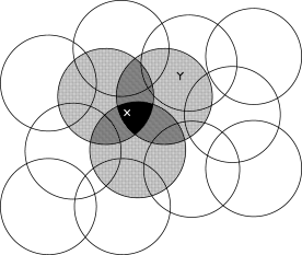
Consider a task in which the state set is continuous and two-dimensional.
A state in this case is a point in 2-space, a vector with two real
components. One kind of feature for this case is
those corresponding to circles in state space, as shown in
Figure
8.2. If the state is inside a circle, then the
corresponding feature has the value ![]() and is said to be present; otherwise the feature is
and is said to be present; otherwise the feature is ![]() and is said to be absent. This kind of 1-0-valued feature is called a binary feature.
Given a state, which binary features are present indicate within
which circles the state lies, and thus coarsely code for its location.
Representing a state with features that overlap in this way
(although they need not be circles or binary) is known as coarse coding.
and is said to be absent. This kind of 1-0-valued feature is called a binary feature.
Given a state, which binary features are present indicate within
which circles the state lies, and thus coarsely code for its location.
Representing a state with features that overlap in this way
(although they need not be circles or binary) is known as coarse coding.
Assuming linear gradient-descent function approximation, consider the
effect of the size and density of the circles. Corresponding to each circle is
a single parameter (a component of ![]() ) that is affected by learning. If we
train at one point (state),
) that is affected by learning. If we
train at one point (state),
![]() , then the parameters of all circles intersecting
, then the parameters of all circles intersecting
![]() will be affected. Thus, by (8.8), the approximate value
function will be affected at all points within the union of the circles,
with a greater effect the more circles a point has "in common" with
will be affected. Thus, by (8.8), the approximate value
function will be affected at all points within the union of the circles,
with a greater effect the more circles a point has "in common" with ![]() , as
shown in Figure
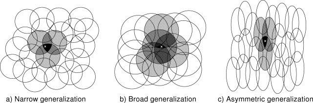
8.2. If the circles are small,
then the generalization will be over a short distance, as in
Figure
8.3a, whereas if they are large, it will be over a
large distance, as in
Figure
8.3b. Moreover, the shape of the features will
determine the nature of the generalization. For example, if they are not
strictly circular, but are elongated in one direction, then generalization
will be similarly affected, as in Figure
8.3c.
, as
shown in Figure
8.2. If the circles are small,
then the generalization will be over a short distance, as in
Figure
8.3a, whereas if they are large, it will be over a
large distance, as in
Figure
8.3b. Moreover, the shape of the features will
determine the nature of the generalization. For example, if they are not
strictly circular, but are elongated in one direction, then generalization
will be similarly affected, as in Figure
8.3c.
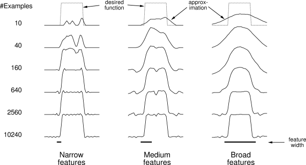
Features with large receptive fields give broad generalization, but might also seem to limit the learned function to a coarse approximation, unable to make discriminations much finer than the width of the receptive fields. Happily, this is not the case. Initial generalization from one point to another is indeed controlled by the size and shape of the receptive fields, but acuity, the finest discrimination ultimately possible, is controlled more by the total number of features.
Example 8.1: Coarseness of Coarse Coding This example illustrates the effect on learning of the size of the receptive fields in coarse coding. Linear function approximation based on coarse coding and (8.3) was used to learn a one-dimensional square-wave function (shown at the top of Figure 8.4). The values of this function were used as the targets,

|
Tile coding is a form of coarse coding that is particularly well suited for use on sequential digital computers and for efficient on-line learning. In tile coding the receptive fields of the features are grouped into exhaustive partitions of the input space. Each such partition is called a tiling, and each element of the partition is called a tile. Each tile is the receptive field for one binary feature.
An immediate advantage of tile coding is that the overall number of
features that are present at one time is strictly controlled and independent
of the input state. Exactly one feature is present in each tiling, so the
total number of features present is always the same as the number of
tilings. This allows
the step-size parameter, ![]() , to be set in an easy, intuitive way. For example,
choosing
, to be set in an easy, intuitive way. For example,
choosing ![]() , where
, where
![]() is the number of tilings, results in exact one-trial learning. If the
example
is the number of tilings, results in exact one-trial learning. If the
example ![]() is received, then whatever the prior value,
is received, then whatever the prior value, ![]() ,
the new value will be
,
the new value will be ![]() . Usually one wishes to change
more slowly than this, to allow for generalization and stochastic variation
in target outputs. For example, one might choose
. Usually one wishes to change
more slowly than this, to allow for generalization and stochastic variation
in target outputs. For example, one might choose
![]() , in which case one would move one-tenth of
the way to the target in one update.
, in which case one would move one-tenth of
the way to the target in one update.
Because tile coding uses exclusively binary (0-1-valued) features, the weighted
sum making up the approximate value function (8.8) is almost trivial
to compute. Rather than performing ![]() multiplications and additions, one simply
computes the indices of the
multiplications and additions, one simply
computes the indices of the
![]() present features and then adds up the
present features and then adds up the ![]() corresponding components of
the parameter vector. The eligibility trace computation (8.7) is
also simplified because the components of the gradient,
corresponding components of
the parameter vector. The eligibility trace computation (8.7) is
also simplified because the components of the gradient,
![]() , are also usually
, are also usually ![]() , and otherwise
, and otherwise ![]() .
.
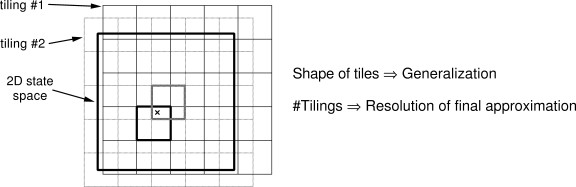
The computation of the indices of the present features is particularly easy if gridlike tilings are used. The ideas and techniques here are best illustrated by examples. Suppose we address a task with two continuous state variables. Then the simplest way to tile the space is with a uniform two-dimensional grid:

|
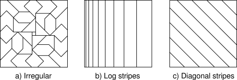
It is important to note that the tilings can be arbitrary and need not be uniform grids. Not only can the tiles be strangely shaped, as in Figure 8.6a, but they can be shaped and distributed to give particular kinds of generalization. For example, the stripe tiling in Figure 8.6b will promote generalization along the vertical dimension and discrimination along the horizontal dimension, particularly on the left. The diagonal stripe tiling in Figure 8.6c will promote generalization along one diagonal. In higher dimensions, axis-aligned stripes correspond to ignoring some of the dimensions in some of the tilings, that is, to hyperplanar slices.
Another important trick for reducing memory requirements is hashing--a consistent pseudo-random collapsing of a large tiling into a much smaller set of tiles. Hashing produces tiles consisting of noncontiguous, disjoint regions randomly spread throughout the state space, but that still form an exhaustive tiling. For example, one tile might consist of the four subtiles shown below:

|
Exercise 8.7 Suppose we believe that one of two state dimensions is more likely to have an effect on the value function than is the other, that generalization should be primarily across this dimension rather than along it. What kind of tilings could be used to take advantage of this prior knowledge?
Radial basis functions (RBFs) are the natural generalization of coarse
coding to continuous-valued features. Rather than each feature being
either 0 or 1, it can be anything in the interval ![]() , reflecting
various degrees to which the feature is present. A typical RBF
feature,
, reflecting
various degrees to which the feature is present. A typical RBF
feature,
![]() , has a Gaussian (bell-shaped) response
, has a Gaussian (bell-shaped) response ![]() dependent only on
the distance between the state,
dependent only on
the distance between the state, ![]() , and the feature's prototypical or
center state,
, and the feature's prototypical or
center state, ![]() , and relative to the feature's width,
, and relative to the feature's width, ![]() :
:

|
An RBF network is a linear function approximator using RBFs for its features. Learning is defined by equations (8.3) and (8.8), exactly as in other linear function approximators. The primary advantage of RBFs over binary features is that they produce approximate functions that vary smoothly and are differentiable. In addition, some learning methods for RBF networks change the centers and widths of the features as well. Such nonlinear methods may be able to fit the target function much more precisely. The downside to RBF networks, and to nonlinear RBF networks especially, is greater computational complexity and, often, more manual tuning before learning is robust and efficient.
On tasks with very high dimensionality, say hundreds of dimensions, tile coding and RBF networks become impractical. If we take either method at face value, its computational complexity increases exponentially with the number of dimensions. There are a number of tricks that can reduce this growth (such as hashing), but even these become impractical after a few tens of dimensions.
On the other hand, some of the general ideas underlying these methods can be practical for high-dimensional tasks. In particular, the idea of representing states by a list of the features present and then mapping those features linearly to an approximation may scale well to large tasks. The key is to keep the number of features from scaling explosively. Is there any reason to think this might be possible?
First we need to establish some realistic expectations. Roughly speaking, a function approximator of a given complexity can only accurately approximate target functions of comparable complexity. But as dimensionality increases, the size of the state space inherently increases exponentially. It is reasonable to assume that in the worst case the complexity of the target function scales like the size of the state space. Thus, if we focus the worst case, then there is no solution, no way to get good approximations for high-dimensional tasks without using resources exponential in the dimension.
A more useful way to think about the problem is to focus on the complexity of the target function as separate and distinct from the size and dimensionality of the state space. The size of the state space may give an upper bound on complexity, but short of that high bound, complexity and dimension can be unrelated. For example, one might have a 1000-dimensional task where only one of the dimensions happens to matter. Given a certain level of complexity, we then seek to be able to accurately approximate any target function of that complexity or less. As the target level of complexity increases, we would like to get by with a proportionate increase in computational resources.
From this point of view, the real source of the problem is the complexity of the target function, or of a reasonable approximation of it, not the dimensionality of the state space. Thus, adding dimensions, such as new sensors or new features, to a task should be almost without consequence if the complexity of the needed approximations remains the same. The new dimensions may even make things easier if the target function can be simply expressed in terms of them. Unfortunately, methods like tile coding and RBF coding do not work this way. Their complexity increases exponentially with dimensionality even if the complexity of the target function does not. For these methods, dimensionality itself is still a problem. We need methods whose complexity is unaffected by dimensionality per se, methods that are limited only by, and scale well with, the complexity of what they approximate.
One simple approach that meets these criteria, which we call Kanerva coding, is to choose binary features that correspond to particular prototype states. For definiteness, let us say that the prototypes are randomly selected from the entire state space. The receptive field of such a feature is all states sufficiently close to the prototype. Kanerva coding uses a different kind of distance metric than in is used in tile coding and RBFs. For definiteness, consider a binary state space and the hamming distance, the number of bits at which two states differ. States are considered similar if they agree on enough dimensions, even if they are totally different on others.
The strength of Kanerva coding is that the complexity of the functions that can be learned depends entirely on the number of features, which bears no necessary relationship to the dimensionality of the task. The number of features can be more or less than the number of dimensions. Only in the worst case must it be exponential in the number of dimensions. Dimensionality itself is thus no longer a problem. Complex functions are still a problem, as they have to be. To handle more complex tasks, a Kanerva coding approach simply needs more features. There is not a great deal of experience with such systems, but what there is suggests that their abilities increase in proportion to their computational resources. This is an area of current research, and significant improvements in existing methods can still easily be found.