An important problem in the operation of a cellular telephone system is how to efficiently use the available bandwidth to provide good service to as many customers as possible. This problem is becoming critical with the rapid growth in the use of cellular telephones. Here we describe a study due to Singh and Bertsekas (1997) in which they applied reinforcement learning to this problem.
Mobile telephone systems take advantage of the fact that a communication channel--a band of frequencies--can be used simultaneously by many callers if these callers are spaced physically far enough apart that their calls do not interfere with each another. The minimum distance at which there is no interference is called the channel reuse constraint. In a cellular telephone system, the service area is divided into a number of regions called cells. In each cell is a base station that handles all the calls made within the cell. The total available bandwidth is divided permanently into a number of channels. Channels must then be allocated to cells and to calls made within cells without violating the channel reuse constraint. There are a great many ways to do this, some of which are better than others in terms of how reliably they make channels available to new calls, or to calls that are "handed off" from one cell to another as the caller crosses a cell boundary. If no channel is available for a new or a handed-off call, the call is lost, or blocked. Singh and Bertsekas considered the problem of allocating channels so that the number of blocked calls is minimized.
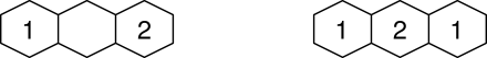
A simple example provides some intuition about the nature of the problem. Imagine a situation with three cells sharing two channels. The three cells are arranged in a line where no two adjacent cells can use the same channel without violating the channel reuse constraint. If the left cell is serving a call on channel 1 while the right cell is serving another call on channel 2, as in the left diagram below, then any new call arriving in the middle cell must be blocked.
|
The simplest approach is to permanently assign channels to cells in such a way that the channel reuse constraint can never be violated even if all channels of all cells are used simultaneously. This is called a fixed assignment method. In a dynamic assignment method, in contrast, all channels are potentially available to all cells and are assigned to cells dynamically as calls arrive. If this is done right, it can take advantage of temporary changes in the spatial and temporal distribution of calls in order to serve more users. For example, when calls are concentrated in a few cells, these cells can be assigned more channels without increasing the blocking rate in the lightly used cells.
The channel assignment problem can be formulated as a semi-Markov
decision process much as the elevator dispatching problem was in the
previous section. A state in the semi-MDP formulation has two components.
The first is the configuration of the entire cellular system that gives for each
cell the usage state (occupied or unoccupied) of each channel for that cell. A
typical cellular system with 49 cells and 70 channels has a staggering
![]() configurations, ruling out the use of
conventional dynamic programming methods. The other state component is an indicator of what kind
of event caused a state transition: arrival, departure, or handoff. This state
component determines what kinds of actions are possible. When a call arrives,
the possible actions are to assign it a free channel or to block it if no
channels are available. When a call departs, that is, when a caller hangs up,
the system is allowed to reassign the channels in use in that cell in an attempt
to create a better configuration. At time
configurations, ruling out the use of
conventional dynamic programming methods. The other state component is an indicator of what kind
of event caused a state transition: arrival, departure, or handoff. This state
component determines what kinds of actions are possible. When a call arrives,
the possible actions are to assign it a free channel or to block it if no
channels are available. When a call departs, that is, when a caller hangs up,
the system is allowed to reassign the channels in use in that cell in an attempt
to create a better configuration. At time ![]() the immediate reward,
the immediate reward, ![]() , is
the number of calls taking place at that time, and the return is
, is
the number of calls taking place at that time, and the return is
This is another problem greatly simplified if treated in terms of afterstates (Section 6.8). For each state and action, the immediate result is a new configuration, an afterstate. A value function is learned over just these configurations. To select among the possible actions, the resulting configuration was determined and evaluated. The action was then selected that would lead to the configuration of highest estimated value. For example, when a new call arrived at a cell, it could be assigned to any of the free channels, if there were any; otherwise, it had to be blocked. The new configuration that would result from each assignment was easy to compute because it was always a simple deterministic consequence of the assignment. When a call terminated, the newly released channel became available for reassigning to any of the ongoing calls. In this case, the actions of reassigning each ongoing call in the cell to the newly released channel were considered. An action was then selected leading to the configuration with the highest estimated value.
Linear function approximation was used for the value function: the
estimated value of a configuration was a weighted sum of features.
Configurations were represented by two sets of features: an availability feature
for each cell and a packing feature for each cell-channel pair. For any
configuration, the availability feature for a cell gave the number of
additional calls it could accept without conflict if the rest of the cells were
frozen in the current configuration. For any given configuration, the packing
feature for a cell-channel pair gave the number of times that channel was
being used in that configuration within a four-cell radius of that cell. All of
these features were normalized to lie between ![]() and 1. A semi-Markov version
of linear TD(0) was used to update the weights.
and 1. A semi-Markov version
of linear TD(0) was used to update the weights.
Singh and Bertsekas compared three channel allocation methods
using a simulation of a ![]() cellular array with 70 channels. The
channel reuse constraint was that calls had to be 3 cells apart to be allowed to
use the same channel. Calls arrived at cells randomly according to Poisson
distributions possibly having different means for different cells, and call
durations were determined randomly by an exponential distribution with a mean of three
minutes. The methods compared were a fixed assignment method (FA), a dynamic
allocation method called "borrowing with directional channel locking" (BDCL), and the
reinforcement learning method (RL). BDCL (Zhang and Yum, 1989) was
the best dynamic channel allocation method they found in the literature. It is a
heuristic method that assigns channels to cells as in FA, but channels can be borrowed
from neighboring cells when needed. It orders the channels in each cell and uses this
ordering to determine which channels to borrow and how calls are dynamically reassigned
channels within a cell.
cellular array with 70 channels. The
channel reuse constraint was that calls had to be 3 cells apart to be allowed to
use the same channel. Calls arrived at cells randomly according to Poisson
distributions possibly having different means for different cells, and call
durations were determined randomly by an exponential distribution with a mean of three
minutes. The methods compared were a fixed assignment method (FA), a dynamic
allocation method called "borrowing with directional channel locking" (BDCL), and the
reinforcement learning method (RL). BDCL (Zhang and Yum, 1989) was
the best dynamic channel allocation method they found in the literature. It is a
heuristic method that assigns channels to cells as in FA, but channels can be borrowed
from neighboring cells when needed. It orders the channels in each cell and uses this
ordering to determine which channels to borrow and how calls are dynamically reassigned
channels within a cell.
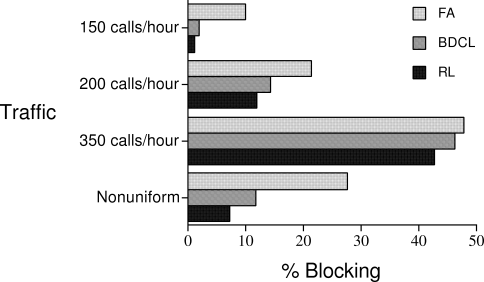
Figure 11.10 shows the blocking probabilities of these methods for mean arrival rates of 150, 200, and 300 calls/hour as well as for a case in which different cells had different mean arrival rates. The reinforcement learning method learned on-line. The data shown are for its asymptotic performance, but in fact learning was rapid. The RL method blocked calls less frequently than did the other methods for all arrival rates and soon after starting to learn. Note that the differences between the methods decreased as the call arrival rate increased. This is to be expected because as the system gets saturated with calls there are fewer opportunities for a dynamic allocation method to set up favorable usage patterns. In practice, however, it is the performance of the unsaturated system that is most important. For marketing reasons, cellular telephone systems are built with enough capacity that more than 10% blocking is rare.
|
Nie and Haykin (1996) also studied the application of reinforcement learning to dynamic channel allocation. They formulated the problem somewhat differently than Singh and Bertsekas did. Instead of trying to minimize the probability of blocking a call directly, their system tried to minimize a more indirect measure of system performance. Cost was assigned to patterns of channel use depending on the distances between calls using the same channels. Patterns in which channels were being used by multiple calls that were close to each other were favored over patterns in which channel-sharing calls were far apart. Nie and Haykin compared their system with a method called MAXAVAIL (Sivarajan, McEliece, and Ketchum, 1990), considered to be one of the best dynamic channel allocation methods. For each new call, it selects the channel that maximizes the total number of channels available in the entire system. Nie and Haykin showed that the blocking probability achieved by their reinforcement learning system was closely comparable to that of MAXAVAIL under a variety of conditions in a 49-cell, 70-channel simulation. A key point, however, is that the allocation policy produced by reinforcement learning can be implemented on-line much more efficiently than MAXAVAIL, which requires so much on-line computation that it is not feasible for large systems.
The studies we described in this section are so recent that the many questions they raise have not yet been answered. We can see, though, that there can be different ways to apply reinforcement learning to the same real-world problem. In the near future, we expect to see many refinements of these applications, as well as many new applications of reinforcement learning to problems arising in communication systems.