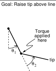
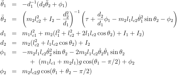
Reinforcement learning has been applied to a wide variety of physical control tasks (e.g., for a collection of robotics applications, see Connell and Mahadevan, 1993). One such task is the acrobot, a two-link, underactuated robot roughly analogous to a gymnast swinging on a high bar (Figure 11.4). The first joint (corresponding to the gymnast's hands on the bar) cannot exert torque, but the second joint (corresponding to the gymnast bending at the waist) can. The system has four continuous state variables: two joint positions and two joint velocities. The equations of motion are given in Figure 11.5. This system has been widely studied by control engineers (e.g., Spong, 1994) and machine-learning researchers (e.g., Dejong and Spong, 1994; Boone, 1997).
One objective for controlling the acrobot is to swing the tip (the "feet")
above the first joint by an amount equal to one of the links in
minimum time. In this task, the torque applied at the second joint is limited to
three choices: positive torque of a fixed magnitude, negative torque of the same
magnitude, or no torque. A reward of ![]() is given on all time steps until the
goal is reached, which ends the episode. No discounting is used (
is given on all time steps until the
goal is reached, which ends the episode. No discounting is used (![]() ). Thus,
the optimal value,
). Thus,
the optimal value, ![]() , of any state,
, of any state,
![]() , is the minimum time to reach the goal (an integer number of steps)
starting from
, is the minimum time to reach the goal (an integer number of steps)
starting from ![]() .
.
Sutton (1996) addressed the acrobot swing-up task in an on-line, modelfree context. Although the acrobot was simulated, the simulator was not available for use by the agent/controller in any way. The training and interaction were just as if a real, physical acrobot had been used. Each episode began with both links of the acrobot hanging straight down and at rest. Torques were applied by the reinforcement learning agent until the goal was reached, which always happened eventually. Then the acrobot was restored to its initial rest position and a new episode was begun.
The learning algorithm used was Sarsa(![]() ) with linear function approximation,
tile coding, and replacing traces as in Figure 8.8. With a small,
discrete action set, it is natural to use a separate set of tilings for each
action. The next choice is of the continuous variables with which to represent
the state. A clever designer would probably represent the state in terms of the
angular position and velocity of the center of mass and of the second link,
which might make the solution simpler
and consistent with broad generalization. But
since this was just a test problem, a more naive, direct representation was used in
terms of the positions and velocities of the links:
) with linear function approximation,
tile coding, and replacing traces as in Figure 8.8. With a small,
discrete action set, it is natural to use a separate set of tilings for each
action. The next choice is of the continuous variables with which to represent
the state. A clever designer would probably represent the state in terms of the
angular position and velocity of the center of mass and of the second link,
which might make the solution simpler
and consistent with broad generalization. But
since this was just a test problem, a more naive, direct representation was used in
terms of the positions and velocities of the links: ![]() , and
, and ![]() . The two angles are restricted to a limited range
by the physics of the acrobot (see Figure
11.5) and the two
angles are naturally restricted to
. The two angles are restricted to a limited range
by the physics of the acrobot (see Figure
11.5) and the two
angles are naturally restricted to ![]() . Thus, the state space in this task
is a bounded rectangular region in four dimensions.
. Thus, the state space in this task
is a bounded rectangular region in four dimensions.
This leaves the question of what tilings to use. There are many possibilities, as discussed in Chapter 8. One is to use a complete grid, slicing the four-dimensional space along all dimensions, and thus into many small four-dimensional tiles. Alternatively, one could slice along only one of the dimensions, making hyperplanar stripes. In this case one has to pick which dimension to slice along. And of course in all cases one has to pick the width of the slices, the number of tilings of each kind, and, if there are multiple tilings, how to offset them. One could also slice along pairs or triplets of dimensions to get other tilings. For example, if one expected the velocities of the two links to interact strongly in their effect on value, then one might make many tilings that sliced along both of these dimensions. If one thought the region around zero velocity was particularly critical, then the slices could be more closely spaced there.
Sutton used tilings that sliced in a variety of simple ways. Each of the four
dimensions was divided into six equal intervals. A seventh interval was added to
the angular velocities so that tilings could be offset by a random fraction of an
interval in all dimensions (see Chapter 8, subsection
"Tile Coding"). Of the total of 48 tilings, 12 sliced along
all four dimensions as discussed above, dividing the space into ![]() tiles each. Another 12 tilings sliced
along three dimensions (3 randomly offset tilings each for each of the 4 sets
of three dimensions), and another 12 sliced along two dimensions (2 tilings for
each of the 6 sets of two dimensions. Finally, a set of 12 tilings
depended each on only one dimension (3 tilings for each of the 4 dimensions). This
resulted in a total of approximately
tiles each. Another 12 tilings sliced
along three dimensions (3 randomly offset tilings each for each of the 4 sets
of three dimensions), and another 12 sliced along two dimensions (2 tilings for
each of the 6 sets of two dimensions. Finally, a set of 12 tilings
depended each on only one dimension (3 tilings for each of the 4 dimensions). This
resulted in a total of approximately
![]() tiles for each action. This number is small enough that hashing was
not necessary. All tilings were offset by a random fraction of an interval in all
relevant dimensions.
tiles for each action. This number is small enough that hashing was
not necessary. All tilings were offset by a random fraction of an interval in all
relevant dimensions.
The remaining parameters of the learning algorithm were
![]() ,
, ![]() ,
, ![]() , and
, and ![]() . The use of a greedy
policy (
. The use of a greedy
policy (![]() ) seemed preferable on this task because long sequences of
correct actions are needed to do well. One exploratory action could spoil a
whole sequence of good actions. Exploration was ensured instead by starting
the action values optimistically, at the low value of 0. As discussed in
Section 2.7 and Example 8.2, this makes the agent continually disappointed with
whatever rewards it initially experiences, driving it to keep trying new things.
) seemed preferable on this task because long sequences of
correct actions are needed to do well. One exploratory action could spoil a
whole sequence of good actions. Exploration was ensured instead by starting
the action values optimistically, at the low value of 0. As discussed in
Section 2.7 and Example 8.2, this makes the agent continually disappointed with
whatever rewards it initially experiences, driving it to keep trying new things.
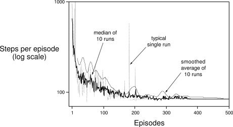
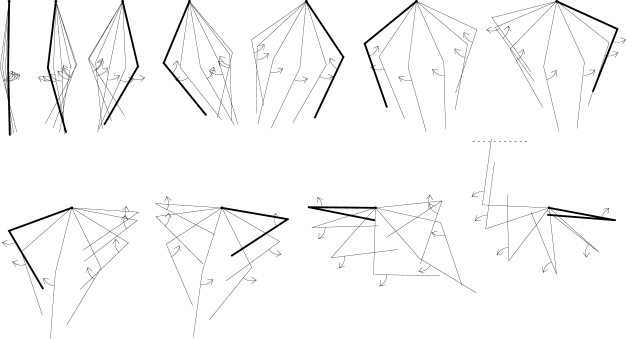
Figure 11.6 shows learning curves for the acrobot task and the learning algorithm described above. Note from the single-run curve that single episodes were sometimes extremely long. On these episodes, the acrobot was usually spinning repeatedly at the second joint while the first joint changed only slightly from vertical down. Although this often happened for many time steps, it always eventually ended as the action values were driven lower. All runs ended with an efficient policy for solving the problem, usually lasting about 75 steps. A typical final solution is shown in Figure 11.7. First the acrobot pumps back and forth several times symmetrically, with the second link always down. Then, once enough energy has been added to the system, the second link is swung upright and stabbed to the goal height.
|