

Next: 2.8 Reinforcement Comparison
Up: 2 Evaluative Feedback
Previous: 2.6 Tracking a Nonstationary
All the methods we have discussed so far are dependent to some extent on the
initial action-value estimates,  . In the language of statistics, these
methods are biased by their initial estimates. For the sample-average
methods, the bias disappears once all actions have been selected at least once, but
for methods with constant
  , the bias is permanent, though decreasing over
time as given by (2.6). In practice, this kind of bias is usually not a
problem, and can sometimes be very helpful. The downside is that the initial
estimates become, in effect, a whole set of parameters that must be picked by
the user, if only to set them all to zero. The upside is that they provide an easy
way to supply some prior knowledge about what level of rewards can be expected.
Initial action values can also be used as a simple way of encouraging exploration.
Suppose that instead of setting the initial action values to zero, as we did in the 10-armed
testbed, we set them all to +5. Recall that the  in this problem
are selected from a normal distribution with mean 0 and variance 1. An initial
estimate of +5 is thus wildly optimistic. But this optimism encourages
action-value methods to explore. Whichever actions are initially selected, the reward
is less than the starting estimates; the learner switches
to other actions, being ``disappointed" with the rewards it is receiving.
The result is that all actions are tried, several times, before the value estimates
converge. The system does a fair amount of exploration even if greedy actions are
selected all the time.

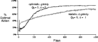
Figure 2.4: The effect of optimistic initial action-values estimates on the
10-armed testbed. Both algorithms used constant step size,  .
.
Figure 2.4 shows the performance on the 10-armed
bandit testbed of a greedy method using  , for all a. For comparison,
also shown is an
  -greedy method with
  . Both methods used a constant
step size,
  . Initially, the optimistic method performs worse, because it
explores more, but eventually it performs better because its exploration decreases
with time. We call this technique for encouraging exploration optimistic
initial values. We regard it as a simple trick that can be quite effective on
stationary problems, but it is far from being a generally useful approach to
encouraging exploration. For example, it is not well suited to nonstationary
problems because its drive for exploration is inherently temporary. If the task
changes, creating a renewed need for exploration, this method cannot help. Indeed,
any method that focuses on the initial state in any special way is unlikely to help
with the general non-stationary case. The beginning of time occurs only once, and
thus we should not focus on it too much. This criticism applies as well to the
sample-average methods, which also treat the beginning of time as a special event,
averaging with equal weights all subsequent rewards. Nevertheless, all of these
methods are very simple, and one or some simple combination of them is often adequate
in practice. In the rest of this book we make frequent use of many of the
exploration techniques that we explore here within the simpler non-associative
setting of the n
-armed bandit problem.
Exercise  .
.
The results shown in Figure 2.4 should be quite reliable because
they are averages over 2000 individual, randomly chosen 10-armed
bandit tasks. Why, then, are there oscillations and spikes in the early part of the
curve for the optimistic method? What might make this method perform
particularly better or worse, on average, on particular early plays?


Next: 2.8 Reinforcement Comparison
Up: 2 Evaluative Feedback
Previous: 2.6 Tracking a Nonstationary
Richard Sutton
Sat May 31 12:02:11 EDT 1997
 . In the language of statistics, these
methods are biased by their initial estimates. For the sample-average
methods, the bias disappears once all actions have been selected at least once, but
for methods with constant
  , the bias is permanent, though decreasing over
time as given by (2.6). In practice, this kind of bias is usually not a
problem, and can sometimes be very helpful. The downside is that the initial
estimates become, in effect, a whole set of parameters that must be picked by
the user, if only to set them all to zero. The upside is that they provide an easy
way to supply some prior knowledge about what level of rewards can be expected.


 in this problem
are selected from a normal distribution with mean 0 and variance 1. An initial
estimate of +5 is thus wildly optimistic. But this optimism encourages
action-value methods to explore. Whichever actions are initially selected, the reward
is less than the starting estimates; the learner switches
to other actions, being ``disappointed" with the rewards it is receiving.
The result is that all actions are tried, several times, before the value estimates
converge. The system does a fair amount of exploration even if greedy actions are
selected all the time.

 .
. , for all a. For comparison,
also shown is an
  -greedy method with
  . Both methods used a constant
step size,
  . Initially, the optimistic method performs worse, because it
explores more, but eventually it performs better because its exploration decreases
with time. We call this technique for encouraging exploration optimistic
initial values. We regard it as a simple trick that can be quite effective on
stationary problems, but it is far from being a generally useful approach to
encouraging exploration. For example, it is not well suited to nonstationary
problems because its drive for exploration is inherently temporary. If the task
changes, creating a renewed need for exploration, this method cannot help. Indeed,
any method that focuses on the initial state in any special way is unlikely to help
with the general non-stationary case. The beginning of time occurs only once, and
thus we should not focus on it too much. This criticism applies as well to the
sample-average methods, which also treat the beginning of time as a special event,
averaging with equal weights all subsequent rewards. Nevertheless, all of these
methods are very simple, and one or some simple combination of them is often adequate
in practice. In the rest of this book we make frequent use of many of the
exploration techniques that we explore here within the simpler non-associative
setting of the n
-armed bandit problem.
 .
.